Comparing Optimization Algorithm Choices in ADMM

This tutorial shows how to compare perfomance of ADDM solver for different optimization algorithm choices. In this example, we will compare Newton-Raphson method, BFGS method and L-BFGS method.

library(solvers)
library(lattice)

# Generating data
n <- 1000
p <- 40
d <- randomProblem(n, p, response = "binomial", density=0.5)
x <- d$x
y <- d$y

Now that we have out training data-set, we will use ADMM to obtain the fit thrice - once with Newton-Raphson as optimization algorithm, once with BFGS as optimization algorithm and finally once with L-BFGS as optimization algorithm. Note that diagnostics=TRUE flag is necessary so that solver records the metrics at each iteration.

# Obtaining the fit for the solvers we want to compare
admm_nr <- ADMM(x, y, family="binomial", opt_algo="nr", alpha=(0.01),diagnostics=TRUE)
admm_bfgs <- ADMM(x, y, family="binomial", opt_algo="bfgs", alpha=(0.01),diagnostics=TRUE)
admm_lbfgs <- ADMM(x, y, family="binomial", opt_algo="lbfgs", alpha=(0.01),diagnostics=TRUE)

To compare total execution time, we can use total_time attribute of the fit.

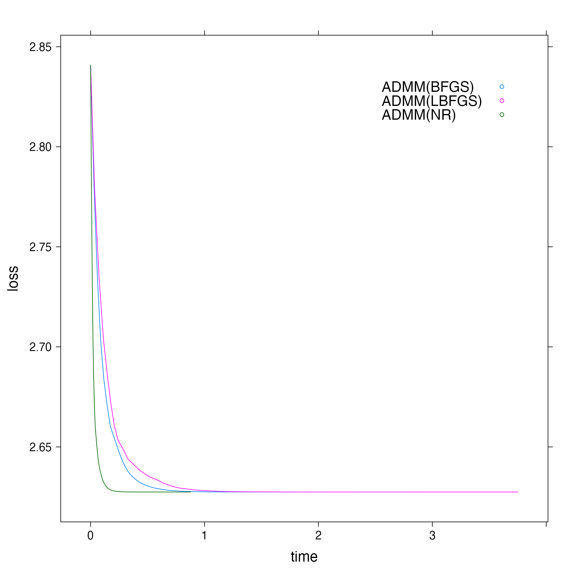
# Comparing total execution time
print(admm_nr$total_time)
#> [1] 0.8868921
print(admm_bfgs$total_time)
#> [1] 2.945276
print(admm_lbfgs$total_time)
#> [1] 3.778316

Now, these fits cannot be directly used to plot as they contain a lot of parameter so we’ll call a utility function that merges the relevant parameter and returns a dataframe.

# Merging the metrics into one dataframe
f <- mergeFits(list(admm_nr, admm_bfgs, admm_lbfgs))

Finally, now we can generate the loss vs time plot.

# Plotting objective vs time
plt <- xyplot(loss ~ time, group = solver, data = f, auto.key = list(corner = c(0.9, 0.9)), type = "l")
update(plt, par.settings = list(fontsize = list(text = 18)))

Akarsh Goyal

2020-08-31